Bayesian inference is statistical inference in which evidence or observations are used to update or to newly infer the probability that a hypothesis may be true. The name "Bayesian" comes from the frequent use of Bayes' theorem in the inference process. Bayes' theorem was derived from the work of the Reverend Thomas Bayes.

Evidence and changing beliefs

From which bowl is the cookie?
False positives result when a test falsely or incorrectly reports a positive result. For example, a medical test for a disease may return a positive result indicating that patient has a disease even if the patient does not have the disease. We can use Bayes' theorem to determine the probability that a positive result is in fact a false positive. We find that if a disease is rare, then the majority of positive results may be false positives, even if the test is accurate.
Suppose that a test for a disease generates the following results:
Suppose also that only 0.1% of the population has that disease, so that a randomly selected patient has a 0.001 prior probability of having the disease.
We can use Bayes' theorem to calculate the probability that a positive test result is a false positive.
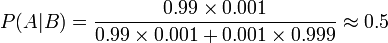
Let A represent the condition in which the patient has the disease, and B represent the evidence of a positive test result. Then, probability that the patient actually has the disease given the positive test result is

and hence the probability that a positive result is a false positive is about  (1 – 0.019) = 0.981.
Despite the apparent high accuracy of the test, the incidence of the disease is so low that the vast majority of patients who test positive do not have the disease. Nonetheless, the fraction of patients who test positive who have the disease (.019) is 19 times the fraction of people who have not yet taken the test who have the disease (.001). Thus the test is not useless, and re-testing may improve the reliability of the result.
In order to reduce the problem of false positives, a test should be very accurate in reporting a negative result when the patient does not have the disease. If the test reported a negative result in patients without the disease with probability 0.999, then
,
so that 1- 0.5 = 0.5 now is the probability of a false positive.
On the other hand, false negatives result when a test falsely or incorrectly reports a negative result. For example, a medical test for a disease may return a negative result indicating that patient does not have a disease even though the patient actually has the disease. We can also use Bayes' theorem to calculate the probability of a false negative. In the first example above,

The probability that a negative result is a false negative is about 0.0000105 or 0.00105%. When a disease is rare, false negatives will not be a major problem with the test.
But if 60% of the population had the disease, then the probability of a false negative would be greater. With the above test, the probability of a false negative would be

The probability that a negative result is a false negative rises to 0.0155 or 1.55%.

If a tested patient has the disease, the test returns a positive result 99% of the time, or with probability 0.99
If a tested patient does not have the disease, the test returns a negative result 95% of the time, or with probability 0.95. False positives in a medical test
Bayesian inference can be used in a court setting by an individual juror to coherently accumulate the evidence for and against the guilt of the defendant, and to see whether, in totality, it meets their personal threshold for 'beyond a reasonable doubt'.
Bayesian inference tells us that if we can assign a probability p(G) to the defendant's guilt before we take the DNA evidence into account, then we can revise this probability to the conditional probability P(G | E), since

Suppose, on the basis of other evidence, a juror decides that there is a 30% chance that the defendant is guilty. Suppose also that the forensic evidence is that the probability that a person chosen at random would have DNA that matched that at the crime scene was 1 in a million, or 10.
The event E can occur in two ways. Either the defendant is guilty (with prior probability 0.3) and thus his DNA is present with probability 1, or he is innocent (with prior probability 0.7) and he is unlucky enough to be one of the 1 in a million matching people.
Thus the juror could coherently revise his opinion to take into account the DNA evidence as follows:
.
The benefit of adopting a Bayesian approach is that it gives the juror a formal mechanism for combining the evidence presented. The approach can be applied successively to all the pieces of evidence presented in court, with the posterior from one stage becoming the prior for the next.
The juror would still have to have a prior for the guilt probability before the first piece of evidence is considered. It has been suggested that this could be the guilt probability of a random person of the appropriate sex taken from the town where the crime occurred. Thus, for a crime committed by an adult male in a town containing 50,000 adult males the appropriate initial prior probability might be 1/50,000.
For the purpose of explaining Bayes' theorem to jurors, it will usually be appropriate to give it in the form of betting odds rather than probabilities, as these are more widely understood. In this form Bayes' theorem states that
Posterior odds = prior odds x Bayes factor
In the example above, the juror who has a prior probability of 0.3 for the defendant being guilty would now express that in the form of odds of 3:7 in favour of the defendant being guilty, the Bayes factor is one million, and the resulting posterior odds are 3 million to 7 or about 429,000 to one in favour of guilt.
In the United Kingdom, Bayes' theorem was explained to the jury in the odds form by a statistician expert witness in the rape case of Regina versus Denis John Adams. A conviction was secured but the case went to Appeal, as no means of accumulating evidence had been provided for those jurors who did not want to use Bayes' theorem. The Court of Appeal upheld the conviction, but also gave their opinion that "To introduce Bayes' Theorem, or any similar method, into a criminal trial plunges the Jury into inappropriate and unnecessary realms of theory and complexity, deflecting them from their proper task." No further appeal was allowed and the issue of Bayesian assessment of forensic DNA data remains controversial.
Gardner-Medwin argues that the criterion on which a verdict in a criminal trial should be based is not the probability of guilt, but rather the probability of the evidence, given that the defendant is innocent. He argues that if the posterior probability of guilt is to be computed by Bayes' theorem, the prior probability of guilt must be known. This will depend on the incidence of the crime and this is an odd piece of evidence to consider in a criminal trial. Consider the following three propositions:
A: The known facts and testimony could have arisen if the defendant is guilty,
B: The known facts and testimony could have arisen if the defendant is innocent,
C: The defendant is guilty.
Gardner-Medwin argues that the jury should believe both A and not-B in order to convict. A and not-B implies the truth of C, but the reverse is not true. It is possible that B and C are both true, but in this case he argues that a jury should acquit, even though they know that they will be letting some guilty people go free.
Other court cases in which probabilistic arguments played some role were the Howland will forgery trial, the Sally Clark case, and the Lucia de Berk case.

Let G be the event that the defendant is guilty.
Let E be the event that the defendant's DNA matches DNA found at the crime scene.
Let P(E | G) be the probability of seeing event E assuming that the defendant is guilty. (Usually this would be taken to be unity.)
Let P(G | E) be the probability that the defendant is guilty assuming the DNA match event E
Let P(G) be the juror's personal estimate of the probability that the defendant is guilty, based on the evidence other than the DNA match. This could be based on his responses under questioning, or previously presented evidence. In the courtroom

Main article: Bayesian search theory Search theory

More mathematical examples
See naive Bayes classifier.

Naive Bayes classifier
In this example we consider the computation of the posterior distribution for the binomial parameter. This is the same problem considered by Bayes in Proposition 9 of his essay.
We are given m observed successes and n observed failures in a binomial experiment. The experiment may be tossing a coin, drawing a ball from an urn, or asking someone their opinion, among many other possibilities. What we know about the parameter (let's call it a) is stated as the prior distribution, p(a).
For a given value of a, the probability of m successes in m+n trials is

Since m and n are fixed, and a is unknown, this is a likelihood function for a. From the continuous form of the law of total probability we have

For some special choices of the prior distribution p(a), the integral can be solved and the posterior takes a convenient form. In particular, if p(a) is a beta distribution with parameters m₀ and n₀, then the posterior is also a beta distribution with parameters m+m₀ and n+n₀.
A conjugate prior is a prior distribution, such as the beta distribution in the above example, which has the property that the posterior is the same type of distribution.
What is "Bayesian" about Proposition 9 is that Bayes presented it as a probability for the parameter a. That is, not only can one compute probabilities for experimental outcomes, but also for the parameter which governs them, and the same algebra is used to make inferences of either kind. Interestingly, Bayes actually states his question in a way that might make the idea of assigning a probability distribution to a parameter palatable to a frequentist. He supposes that a billiard ball is thrown at random onto a billiard table, and that the probabilities p and q are the probabilities that subsequent billiard balls will fall above or below the first ball. By making the binomial parameter a depend on a random event, he cleverly escapes a philosophical quagmire that was an issue he most likely was not even aware of.

Computer applications

On-line textbook: Information Theory, Inference, and Learning Algorithms, by David MacKay, has chapters on Bayesian methods, including examples; arguments in favour of Bayesian methods (in the style of Edwin Jaynes); modern Monte Carlo methods, message-passing methods, and variational methods; and examples illustrating the connections between Bayesian inference and data compression.
Berger, J.O. (1999) Statistical Decision Theory and Bayesian Statistics. Second Edition. Springer Verlag, New York. ISBN 0-387-96098-8 and also ISBN 3-540-96098-8.
Bolstad, William M. (2004) Introduction to Bayesian Statistics, John Wiley ISBN 0-471-27020-2
Bretthorst, G. Larry, 1988, Bayesian Spectrum Analysis and Parameter Estimation in Lecture Notes in Statistics, 48, Springer-Verlag, New York, New York
Dawid, A.P. and Mortera, J. (1996) Coherent analysis of forensic identification evidence. Journal of the Royal Statistical Society, Series B, 58,425-443.
Foreman, L.A; Smith, A.F.M. and Evett, I.W. (1997). Bayesian analysis of deoxyribonucleic acid profiling data in forensic identification applications (with discussion). Journal of the Royal Statistical Society, Series A, 160, 429-469.
Gardner-Medwin, A. What probability should the jury address?. Significance. Volume 2, Issue 1, March 2005
Gelman, A., Carlin, B., Stern, H., and Rubin, D.B. (2003). Bayesian Data Analysis. Second Edition. Chapman & Hall/CRD, Boca Raton, Florida. ISBN 1-58488-388-X.
Gelman, A. and Meng, X.L. (2004). Applied Bayesian Modeling and Causal Inference from Incomplete-Data Perspectives: an essential journey with Donald Rubin's statistical family. John Wiley & Sons, Chichester, UK. ISBN 0-470-09043-X
Jaynes, E.T. (1998) Probability Theory: The Logic of Science.
Lee, Peter M. Bayesian Statistics: An Introduction. Second Edition. (1997). ISBN 0-340-67785-6.
O'Hagan, A. and Forster, J. (2003) Kendall's Advanced Theory of Statistics, Volume 2B: Bayesian Inference. Arnold, New York. ISBN 0-340-52922-9.
Pearl, J. (1988) Probabilistic Reasoning in Intelligent Systems, San Mateo, CA: Morgan Kaufmann.
Robert, C.P. (2001) The Bayesian Choice. Springer Verlag, New York.
Robertson, B. and Vignaux, G.A. (1995) Interpreting Evidence: Evaluating Forensic Science in the Courtroom. John Wiley and Sons. Chichester.
Winkler, Robert L, Introduction to Bayesian Inference and Decision, 2nd Edition (2003) Probabilistic. ISBN 0-9647938-4-9